Reading: The Split-Apply-Combine Strategy for Data Analysis
As part of the course Stat 585X I am taking this semester, I will be posting a series of responses to assigned course readings. Mostly these will be my rambling thoughts as I skim papers.
This week we are reading “The Split-Apply-Combine Strategy for Data Analysis” by Hadley Wickham, published in the Journal of Statistical Software, April 2011, Volume 40, Issue 1. This paper details the split-apply-combine strategy in data analysis and its implementation in R in a package called plyr.
Split-Apply-Combine
I posit that the split-apply-combine strategy is useful in a much larger realm than data analysis. I liken it to the idea of ‘divide and conquer’. The idea is to split up a large task into smaller, bite-sized chunks, apply the solution on each piece independently, and then combine these little pieces back into the final result. Of course, we can accomplish this with base R functions, but plyr provides a very intuitive command structure and naming consistency, not to mention it lessens the number of lines of code I have to write.
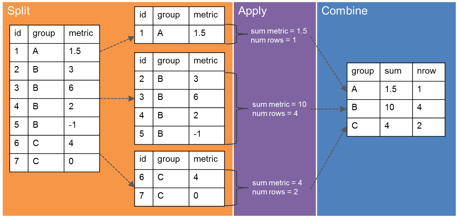
So what does it truly mean to split-combine-apply? What are we splitting? The easiest way I can illustrate the idea is with the concept of a data frame. Imagine we have a data frame with three columns: an identity, a group, and a metric. We may want to know how many identities there are in each group, or maybe we want to know the sum of the metric values within each group. The split-apply-combine strategy will allow us to do this in the following manner:
It’s easiest to conceptualize plyr-ing a data frame because it’s two dimensional. Of course, we can apply the split-apply-combine strategy to objects of more than one dimension. Hadley explains this idea very thoroughly with great images in the paper and I recommend the read if you are using more complicated data structures.
From what to what?
As I mentioned, one of my favorite things about the plyr package is its intuitive naming structure. The way the functions within the package are named defines what data structure is being split [input] and then what format to combine the results into [output]. More specificaly, the functions used to split-apply-combine are names as [input letter][output letter]ply. There are three structures you can use as either input or output.
- Arrays – letter: a
- Data frames – letter: d
- Lists – letter: l
The type of input determines how the opject can be split and what kind of functions can be applied. For example, ddply takes a data frame as input and returns a data frame as output. This naming convention reduced confusion and time spent re-looking up helpfiles when I try to plyr.
Tips Example
To show off the ease of the plyr solutions, I’d like to walk through a small example using the tips dataset from the reshape2 package. This is a dataset with recorded information about each tip he received over a period of a few months working in one restaurant.
library(reshape2)
head(tips)
## total_bill tip sex smoker day time size
## 1 16.99 1.01 Female No Sun Dinner 2
## 2 10.34 1.66 Male No Sun Dinner 3
## 3 21.01 3.50 Male No Sun Dinner 3
## 4 23.68 3.31 Male No Sun Dinner 2
## 5 24.59 3.61 Female No Sun Dinner 4
## 6 25.29 4.71 Male No Sun Dinner 4Let’s say we want to look at average tips earned on Fridays for the server. We could employ a subset strategy, like so:
mean(subset(tips, day == 'Fri')$tip)## [1] 2.734737But what about average tips for each day? I wouldn’t want to have to do each day by hand. Instead, let’s use plyr!
library(plyr)

ddply(tips, .(day), summarise, mean=mean(tip))
## day mean
## 1 Fri 2.734737
## 2 Sat 2.993103
## 3 Sun 3.255132
## 4 Thur 2.771452In the function call you can see we are specifying day to be the group variable and then we want to ‘summarise’ our dataset my displaying the mean tip for each day. We can also easily break this out by meal type.
ddply(tips, .(day, time), summarise, mean=mean(tip))## day time mean
## 1 Fri Dinner 2.940000
## 2 Fri Lunch 2.382857
## 3 Sat Dinner 2.993103
## 4 Sun Dinner 3.255132
## 5 Thur Dinner 3.000000
## 6 Thur Lunch 2.767705From here it’s easy to see that larger tips happen at dinner and the server actually received his largest tips at dinner.
This is a small example of what we can do easily with plyr. But there is a vast expanse of things I haven’t even touched on.
Something new
I have been using plyr for over a year now, but I learned something completely new from reading Hadley’s paper. I didn’t know that you can use formulas and renaming in the variable call to plyr. For example, say we wanted to group by “time_day” and call it “time” for whatever reason. This is possible with the same simple syntax.
ddply(tips, .(time = paste(time, day, sep="_")), summarise, mean=mean(tip))## time mean
## 1 Dinner_Fri 2.940000
## 2 Dinner_Sat 2.993103
## 3 Dinner_Sun 3.255132
## 4 Dinner_Thur 3.000000
## 5 Lunch_Fri 2.382857
## 6 Lunch_Thur 2.767705I know this is a completely contrived example, but I think this little nugget of knowledge could be really useful to me in the future.
Commentary
I hope you get some good mileage out of the split-apply-combine strategy. I use it all the time and really enjoyed reading this paper to learn more deeply about the ideas underlying the plyr package. Let me know in the comments section how plyr is working for you!
blog comments powered by Disqus