Reading: Hierarchical Clustering
As part of the course Stat 503 I am taking this semester, I will be posting a series of responses to assigned course readings and videos. Mostly these will be my rambling thoughts as I skim papers.
This week we reading some documents on clustering methods from Steven Holland (link) and J. C. Wang (link). These readings give a good introduction to the concepts behind hierarchical cluster analysis, including dendrograms, agglomerative methods, and divisive methods.
Introduction
From Holland’s leacture, cluster analysis can be thought of as two sets of techniques: partitioning and hierarchical clustering. Both methods are designed to find groups of similar items within the dataset, but partition divides the dataset into a pre-designated number of groups, while hierarchical methods create a hierarchy of clusters either by combining small groups (agglomerative) or splitting large ones (divisive).
In a hierarchical approach, we can inspect a tree plot known as a dendrogram that shows the structure and how groups are combined or divided. By inspecting a dendrogram, it can become apparent where to split the tree by loking for large distances from one level of splitting to the next. In this way, hierarchical methods are not limited to a pre-determined number of clusters (like partitioning methods).
Wang breaks down clustering into four distinct steps corresponding to the following questions.
Partitioning (forming clusters)
- What variables are used to compute similarity (or distance) among objects?
- How to define similarity (or distance) measure?
- What algorithm should be used to place similar objects into clusters?
- How many clusters should be formed?
It is very important to answer these questions before clustering, because in many cases fitting multiple options can lead to more confusion rather than clarity. For an example of how to answer one of the above questions (3.), we can look at the order in which clusters are joined, controlled by the linkage methods. There are many options available for linkage. The single-linkage method is based on the elements of two clusters that are most similar, and complete-linkage method is based on the elements that are most dissimilar. The median, group average, and centroid methods all emphasize the central tendency of clusters. Lastly, Ward’s method joins clusters based on minimizing the within-group sum of squares. One should choose a linkage method based on a desired trait: single and complete linkage are based on outliers, which may be important for catching extreme cases. The central tendency linkages are less sensitive to outliers, which may be useful. Finally, Ward’s method tends to produce compact clusters.
Example
To get a better feel for how agglomorative hierarchical clustering can be done in R, I’m going to run through an example of clustering cake recipes by ingredients. In this example, we are looking to find groups of similar cakes based on the ingredients that go into making them. The data is available from the package cluster.datasets.
library(cluster.datasets)
library(dplyr)
library(tidyr)
library(ggplot2)
library(knitr)

data(cake.ingredients.1961)
summary(cake.ingredients.1961)
## Cake AE BM BP
## Length:18 Min. :0.250 Min. : NA Min. :0.750
## Class :character 1st Qu.:0.375 1st Qu.: NA 1st Qu.:1.500
## Mode :character Median :0.500 Median : NA Median :3.000
## Mean :0.750 Mean :NaN Mean :2.393
## 3rd Qu.:1.000 3rd Qu.: NA 3rd Qu.:3.000
## Max. :1.500 Max. : NA Max. :4.000
## NA's :15 NA's :18 NA's :11
## BR BS CA CC
## Min. :0.12 Min. :3 Min. : 0.300 Min. :0.20
## 1st Qu.:0.25 1st Qu.:3 1st Qu.: 2.725 1st Qu.:0.50
## Median :0.60 Median :3 Median : 5.150 Median :0.50
## Mean :0.56 Mean :3 Mean : 5.150 Mean :0.84
## 3rd Qu.:0.85 3rd Qu.:3 3rd Qu.: 7.575 3rd Qu.:1.50
## Max. :1.00 Max. :3 Max. :10.000 Max. :1.50
## NA's :11 NA's :17 NA's :16 NA's :13
## CE CI CS CT DC
## Min. :3.00 Min. :1 Min. :0.300 Min. :1.25 Min. :3
## 1st Qu.:3.25 1st Qu.:1 1st Qu.:0.975 1st Qu.:1.25 1st Qu.:3
## Median :3.50 Median :1 Median :1.650 Median :1.25 Median :3
## Mean :3.50 Mean :1 Mean :1.650 Mean :1.25 Mean :3
## 3rd Qu.:3.75 3rd Qu.:1 3rd Qu.:2.325 3rd Qu.:1.25 3rd Qu.:3
## Max. :4.00 Max. :1 Max. :3.000 Max. :1.25 Max. :3
## NA's :16 NA's :17 NA's :16 NA's :17 NA's :17
## EG EY EW FR GN
## Min. :1.000 Min. :2 Min. :10 Min. :0.250 Min. :1.00
## 1st Qu.:2.000 1st Qu.:2 1st Qu.:10 1st Qu.:1.000 1st Qu.:1.25
## Median :3.000 Median :2 Median :10 Median :1.750 Median :1.50
## Mean :3.133 Mean :2 Mean :10 Mean :1.683 Mean :1.50
## 3rd Qu.:4.000 3rd Qu.:2 3rd Qu.:10 3rd Qu.:2.000 3rd Qu.:1.75
## Max. :6.000 Max. :2 Max. :10 Max. :3.000 Max. :2.00
## NA's :3 NA's :16 NA's :17 NA's :3 NA's :16
## HC LJ LR MK NG
## Min. :1.000 Min. :1 Min. :0.5 Min. :0.2500 Min. :1.5
## 1st Qu.:1.000 1st Qu.:1 1st Qu.:1.0 1st Qu.:0.5000 1st Qu.:1.5
## Median :1.000 Median :1 Median :1.0 Median :1.0000 Median :1.5
## Mean :1.333 Mean :1 Mean :0.9 Mean :0.7444 Mean :1.5
## 3rd Qu.:1.500 3rd Qu.:1 3rd Qu.:1.0 3rd Qu.:1.0000 3rd Qu.:1.5
## Max. :2.000 Max. :1 Max. :1.0 Max. :1.0000 Max. :1.5
## NA's :15 NA's :15 NA's :13 NA's :9 NA's :17
## NS RM SA SC SG
## Min. :1 Min. :1.00 Min. :0.5000 Min. :1 Min. : 0.30
## 1st Qu.:1 1st Qu.:1.25 1st Qu.:0.8750 1st Qu.:1 1st Qu.: 0.45
## Median :1 Median :1.50 Median :1.0000 Median :1 Median : 0.75
## Mean :1 Mean :1.50 Mean :0.9375 Mean :1 Mean : 2.95
## 3rd Qu.:1 3rd Qu.:1.75 3rd Qu.:1.0625 3rd Qu.:1 3rd Qu.: 3.25
## Max. :1 Max. :2.00 Max. :1.2500 Max. :1 Max. :10.00
## NA's :17 NA's :16 NA's :14 NA's :14 NA's :14
## SR SS ST VE
## Min. :0.130 Min. :1 Min. :0.2500 Min. :1.000
## 1st Qu.:0.750 1st Qu.:1 1st Qu.:0.2500 1st Qu.:1.000
## Median :1.000 Median :1 Median :0.5000 Median :1.000
## Mean :1.093 Mean :1 Mean :0.5667 Mean :1.222
## 3rd Qu.:1.500 3rd Qu.:1 3rd Qu.:0.8750 3rd Qu.:1.000
## Max. :2.000 Max. :1 Max. :1.0000 Max. :2.000
## NA's :1 NA's :16 NA's :3 NA's :9
## WR YT ZH
## Min. :0.2500 Min. :0.6 Min. :6
## 1st Qu.:0.2500 1st Qu.:0.7 1st Qu.:6
## Median :0.5000 Median :0.8 Median :6
## Mean :0.6071 Mean :0.8 Mean :6
## 3rd Qu.:0.5000 3rd Qu.:0.9 3rd Qu.:6
## Max. :2.0000 Max. :1.0 Max. :6
## NA's :11 NA's :16 NA's :17#replace NA with 0 for not required ingredients
dat.cake <- apply(cake.ingredients.1961, 2, function(col){
col[is.na(col)] <- 0
return(col)
})
dat.cake %>%
data.frame() %>%
mutate_each(funs(as.numeric), -Cake) %>%
mutate_each(funs(scale), -Cake) -> dat.cake #standardize columns for hclust
clust.euc.single <- hclust(dist(dat.cake[, -1], method = "euclidean"), method = "single")
clust.euc.complete <- hclust(dist(dat.cake[, -1], method = "euclidean"), method = "complete")
clust.euc.centroid <- hclust(dist(dat.cake[, -1], method = "euclidean"), method = "centroid")
clust.euc.ward <- hclust(dist(dat.cake[, -1], method = "euclidean"), method = "ward.D2")
plot(clust.euc.single)
plot(clust.euc.complete)
plot(clust.euc.centroid)
plot(clust.euc.ward)
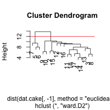
abline(h = 12, col = "red")


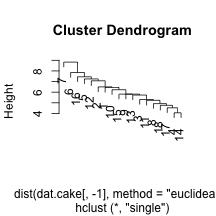
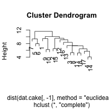
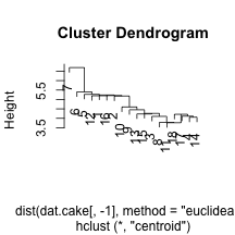
I’ve chosen to look at eucliden distance for the cake ingredients and four distinct linkage mechanisms. Personally, I would want to use Wards to get some nice compact clusters, but it may be useful to see other methods. We can see that the single linkage appears to chain the clusters, adding an element within the same cluster over an over. The centroid does something similarly, but not as extreme. Finally, complete and Ward’s method of linkage appear to add elements to the clusters in a more even keeled manner. For the Ward’s method, I’ve chosen to split into two clusters by drawing a horizontal line at a height of 12. This leavs us with he following two sets of cake clusters.
cake.tree <- cutree(clust.euc.ward, h = 12)
as.character(dat.cake[cake.tree == 1, "Cake"])
## [1] "Angel " "Babas au Rhum "
## [3] "Sweet Chocolate " "Buche de Noel "
## [5] "One Bowl Chocolate " "Red Devil's Food "
## [7] "Sour Cream Fudge " "Hungarian Cream "
## [9] "Crumb and Nut " "Spiced Pound "
## [11] "Strawberry Roll " "Savarin "
## [13] "Banana Shortcake " "Strawberry Shortcake "
## [15] "Sponge "as.character(dat.cake[cake.tree == 2, "Cake"])## [1] "Cheesecake " "Rum Cheesecake " "Blender Cheesecake "It is evident that our custering mechanism was able to split the cheesecakes from the other cakes, which tells me that cheesecake is a fundamentally different kind of cake (and maybe explains why I don’t like it very much).
blog comments powered by Disqus