Regression with Count Data: Theory
The set up: You’ve been asked to find the relationship between n variables. You automatically think REGRESSION! Of course you’re right. and if you’re like me, you think Multivariate Linear Regression should do the trick. This is where the hitch is. Your dependent variable is a count (0,1,2,3,\(\dots\\))! Surely this violates some sort of Ordinary Least Squares assumption, right? What now?
The solution: Count data regression is as simple as linear regression, it just requires a different model. The obvious model from statistics is the Poisson with mean \(\lambda\). Why is this an obvious model? Let’s see how the Poisson distribution fits over some sample count data:
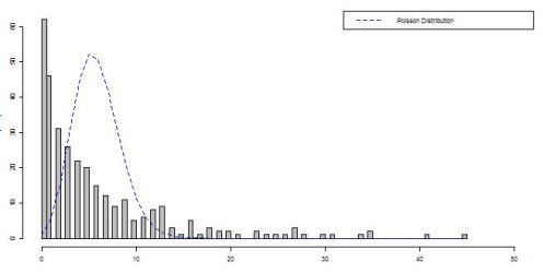
You can see the distribution fits (maybe not the best fit, but what do you expect with the simplest model?) and we can move on to talk about how the model is structured.
The Model: The Poisson regression model takes a general form:
\[\text{E[}y_i\vert x_i\text{]} = \lambda_i = \text{exp (} \beta_1 + \beta_2 x_{2i} + \dots + \beta_k x_{ki})\]Compare the Poisson regression model to the a general linear regression model:
\[\text{E[}y_i\vert x_i] = \mu_i = \beta_1 + \beta_2 x_{2i} + \dots + \beta_k x_{ki}.\]As you can see, the Poisson model can be easily transformed to the linear regression model by taking the natual log of the whole equation: \(\text{ln E[}y_i\vert x_i]=\text{ln} \lambda_i = \text{ln exp}(\beta_1 + \beta_2 x_{2i} + \dots + \beta_k x_{ki}) = \beta_1 + \beta_2 x_{2i} + \dots + \beta_k x_{ki} = \mu_i\)
Thus the Poisson regression model is sometimes called the log-linear model.
Interpretation of Coefficients: The interpretation of the coefficients \(\beta_j\) for the Poisson model is fundamentally different from the interpretation of coefficients in the linear regression model. This is due to the exponentiation present in the Poisson model.
If you think about interpreting the coefficients this way: “What does a one unit change in the jth regressor do to the mean?”, then some calculus and algebra are necessary:
\[\frac{\delta \text{E}[y_i\vert x_i]}{\delta x_{ji}} = \frac{\delta[ \text{exp}(\beta_1 + \beta_2 x_{2i} + \dots + \beta_k x_{ki})]}{\delta x_{ji}} = \beta_j \text{exp}(\beta_1 + \beta_2 x_{2i} + \dots + \beta_k x_{ki}) = \beta_j \text{E}[y_i\vert x_i]\]This tells us that with every one unit change in the jth regressor, there is a change in the mean by the amount \(\beta_j E[y_i\vert x_i]\). For reference, the linear model’s mean would simply change by \(\beta_j\).
Alternative Count Models: The Poisson model, while simple to use and easy to remember does have its draw backs. Namely, it restricts the variance to equal the mean, called equidispersion. Of course, this assumption doesn’t necessarily hold in your data. The data is called overdispersed if the variance exceeds the mean and underdispersed if the variance is less than the mean. Unless the count data is equidispersed, the Poisson model leads to innacurate results.
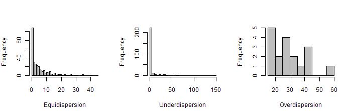
A common, more general model is the Negative Binomial model. The Poisson distribution is simply one case of the Negative Binomial distribution. So, Negative Binomial regression is performed in much the same manner as Poisson, but with more flexibility. This model can be used when the data is overdispersed, but not underdispersed.
If your data is underdispersed, a common solution is to use a Hurdle model. This model treats the process for zeros differently than that for non-zero counts, allowing for a closer fit on zero-inflated data.
Well, that’s a pretty short introduction to the world of Count Data Regression. If you’re interested in learning more, check out Essentials of Count Data Regression or Resources for Count Data Regression both provided by Cameron and Trivedi.
Also, be on the look out for an example of working with count data!
blog comments powered by Disqus