Reading: Dates and Times Made Easy with lubridate
As part of the course Stat 585X I am taking this semester, I will be posting a series of responses to assigned course readings. Mostly these will be my rambling thoughts as I skim papers.
This week we had the pleasure of reading “Dates and Times Made Easy with lubridate” by Garrett Grolemund and Hadley Wickham, published in the Journal of Statistical Software, April 2011, Volume 40, Issue 3. This paper presents an R package called lubridate that facilitates working with dates and times. There are four time related objects introduced in lubridate that are very intuitive: instants, intervals, durations, and periods.
- instants: a specific moment in time, such as January 1st, 2012
- intervals: a span of time that occurs between two specific instants and is always associated with its start and end dates
- durations: a generic time span measured in seconds
- periods: a time span in units larger than seconds, such as years, months, weeks, days, hours, and minutes
With the creation of these four concepts, lubridate offers a flexible and easy way to use date and time in analyses. For a simple idea of what is possible, let us find out what day of the week my birthday will fall on this year.
library(lubridate)
wday(ymd('2014-10-22'), label=TRUE, abbr=FALSE)
## [1] Wednesday
## 7 Levels: Sunday < Monday < Tuesday < Wednesday < Thursday < ... < SaturdayHump day, well that’s a bummer.
Time Zones
Something great that lubridate has functionality for is handling time zones and daylight savings time. For example, as I write this blog post I can find out what time it is in Hawaii, where they are playing the NFL Pro-bowl tonight.
with_tz(Sys.time())## [1] "2016-08-10 10:42:28 CDT"with_tz(Sys.time(), "Pacific/Honolulu")## [1] "2016-08-10 05:42:28 HST"Arithmetic
The time objects in lubridate facilitate arithmetic with dates and times. For a quick example let’s look at flu data from Google that gives an indicator of the current status on flu incidences across states and the nation. Say we want to look at the average value of the past two weeks. This is doable using lubridate.
library(reshape2)
library(plyr)
library(ggplot2)

flu.dat <- read.table("https://www.google.org/flutrends/about/data/flu/us/data.txt", sep=",", header=TRUE, skip=11)
flu.m <- melt(flu.dat[,1:53], id.vars=c('Date')) #only care about states
flu.m <- subset(flu.m, variable != 'United.States') #remove US

flu.m$Date <- ymd(as.character(flu.m$Date))

flu.order <- ddply(subset(flu.m, Date >= max(flu.m$Date) - weeks(2)),.(variable), summarise, avg_2weeks=mean(value))
Then we could look at plots ordered by this average value over the past two week and see what states are having similar flu levels in the last two weeks.
flu.copy <- merge(flu.m, flu.order, all.x=TRUE)
flu.copy$variable <- factor(flu.copy$variable, levels=as.character(flu.order[with(flu.order, order(-avg_2weeks)),"variable"]))
ggplot(flu.copy) + geom_line(aes(x=Date, y=value, group=variable)) + facet_wrap(~variable, nrow=11)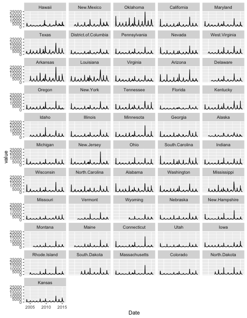 Without lubridate, grappling with the arithmetic of going back 2 weeks would have been painful. I like to avoid painful time arithmetic, so I’m happy to know my way around lubridate.
blog comments powered by Disqus