Reading: datadr - Divide and Recombine in R
As part of the course Stat 585X I am taking this semester, I will be posting a series of responses to assigned course readings. Mostly these will be my rambling thoughts as I skim papers.
This week we are reading documentation on the datadr package by Ryan Hafen from February 2014. This tutorial lay outs the introduction to the new package datadr as well as some background on the Divide-Recombine strategy that the package is built upon.
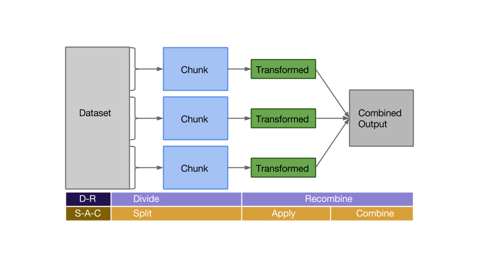
Divide and Recombine (or is it S-A-C?)
The divide and recombine (D-R) strategy is very similar to something we have talked about recently: the Split-Apply-Combine paradigm. In fact, the two seem almost identical. The D-R strategy is to take a dataset, split it in a logical way into many chunks (divide) and then fit them back together after applying some transformation or summary (recombine). Sound familiar? This is the same idea as the S-A-C paradigm, except recombine encompasses both the apply and combine steps.
Birds of a feather…
So we have a package (datadr) based on the D-R strategy and multiple packages (plyr, dplyr) based on the S-A-C paradigm, which are essentially the same thing. What’s the difference between the packages? I would say in some ways datadr is more similar to dplyr than plyr, because
- In datadr, divisions are data objects that persist. The authors did this because with very large data, computing a division is expensive compared to recombination. This is similar to dplyr in that we can create an object with the group_by() function that persists. Often we will use the chaining methods with the %>% operator, but if splitting is an expensive operation and we may want to use the splits with different apply statements, keeping the splits around makes sense.
- Both datadr and dplyr allow for use of the same interface with different backends. For example, dplyr is easily used with data in R memory, or with data from a MySQL, SQLite, or postgreSQL database. Similarly, datadr can be used with data in R memory, or with data in a Hadoop Distributed File System (HDFS), RHIPE, or Hadoop MapReduce setup. Since datadr is already compatible with Hadoop, it would appear that this package has the one up on being able to handle truly huge datasets.
However, datadr uses key-value pairs as its underlying data structure, which can be arranged in list form. dplyr is limited to using a data frame input and output. In this way datadr has some similarity to the plyr package.
Side-by-side example
Let’s take a look at an example of using both datadr and dplyr to accomplish the same task. The data is adult income from the 1994 census database, pulled from the (UCI machine learning repository)[http://archive.ics.uci.edu/ml/datasets/Adult].
We’ll start with the datadr package.
#library(devtools)
#install_github("datadr", "hafen")
library(datadr)
data(adult)

# turn adult into a ddf
(adultDdf <- ddf(adult, update=TRUE))
##
## Distributed data frame backed by 'kvMemory' connection
##
## attribute | value
## ----------------+-----------------------------------------------------------
## names | age(int), workclass(fac), fnlwgt(int), and 13 more
## nrow | 32561
## size (stored) | 2.12 MB
## size (object) | 2.12 MB
## # subsets | 1
##
## * Other attributes: getKeys(), splitSizeDistn(), splitRowDistn(), summary()names(adultDdf)## [1] "age" "workclass" "fnlwgt" "education"
## [5] "educationnum" "marital" "occupation" "relationship"
## [9] "race" "sex" "capgain" "caploss"
## [13] "hoursperweek" "nativecountry" "income" "incomebin"library(ggplot2)
edTable <- summary(adultDdf)$education$freqTable
edTable$var <- with(edTable, reorder(value, Freq, mean))
qplot(var, Freq, data=edTable, geom="point") + coord_flip()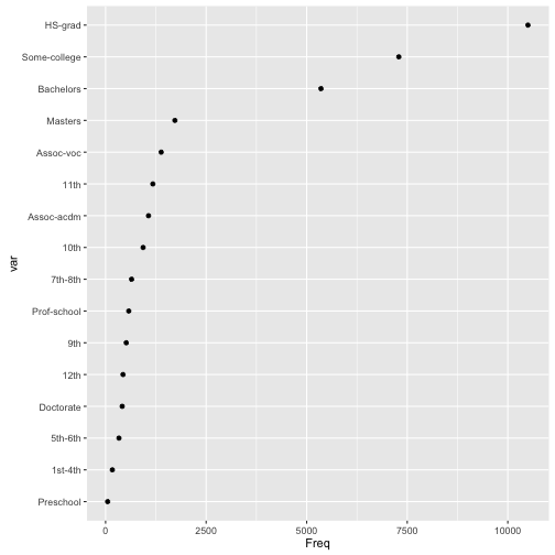 Let’s group the grades together where appropriate and remove preschool. We can make these changes to the education variable within the divide() function. Of course, we could do this to the original data in this case, but this is an illustration. For very large data, it would make more sense (read: be possible) to apply any transformations during the division.
datadr_test <- function() {
  # make a preTransFn to group some education levels
  edGroups <- function(v) {
    v$edGroup <- as.character(v$education)
    v$edGroup[v$edGroup %in% c("1st-4th", "5th-6th")] <- "Some-elementary"
    v$edGroup[v$edGroup %in% c("7th-8th", "9th")] <- "Some-middle"
    v$edGroup[v$edGroup %in% c("10th", "11th", "12th")] <- "Some-HS"
    v
  }

  # divide by edGroup and filter out "Preschool"
  byEdGroup <- divide(addTransform(adultDdf, edGroups), by="edGroup",
                      filterFn=function(x) x$edGroup[1] != "Preschool",
                      update=TRUE)

  print(byEdGroup)

  # tabulate number of people in each education group
  nrowTransform <- function(key, val) {
    newval <- nrow(val)
    kvPair(key, newval)
  }

  edGroupTable <- recombine(addTransform(byEdGroup, nrowTransform), combine=combRbind())
  print(edGroupTable)

  #order for plotting
  edGroupTable$edGroup <- with(edGroupTable, reorder(edGroup, val, mean))
  print(qplot(edGroup, val, data=edGroupTable, geom="point") + coord_flip())
}
datadr_test()
## *** finding global variables used in 'fn'...## [none]## *** testing 'fn' on a subset...## ok## * Verifying parameters...## * Applying division...## * Running map/reduce to get missing attributes...##
## Distributed data frame backed by 'kvMemory' connection
##
## attribute | value
## ----------------+-----------------------------------------------------------
## names | age(int), workclass(cha), fnlwgt(int), and 13 more
## nrow | 32510
## size (stored) | 3.3 MB
## size (object) | 3.3 MB
## # subsets | 11
##
## * Other attributes: getKeys(), splitSizeDistn(), splitRowDistn(), summary()
## * Conditioning variables: edGroup## * Applying recombination...## *** finding global variables used in 'fn'...## [none]## package dependencies: datadr## *** testing 'fn' on a subset...## ok## edGroup val
## 1 Assoc-acdm 1067
## 2 Assoc-voc 1382
## 3 Bachelors 5355
## 4 Doctorate 413
## 5 HS-grad 10501
## 6 Masters 1723
## 7 Prof-school 576
## 8 Some-college 7291
## 9 Some-elementary 501
## 10 Some-HS 2541
## 11 Some-middle 1160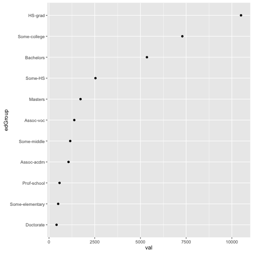
Now let’s do the same thing with dplyr.
library(dplyr)
dplyr_test <- function() {
  byEdGroup_dplyr <- adult %>%
    mutate(edGroup = ifelse(as.character(education) %in% c("1st-4th", "5th-6th"), "Some-elementary",
                            ifelse(as.character(education) %in% c("7th-8th", "9th"), "Some-middle",
                                   ifelse(as.character(education) %in% c("10th", "11th", "12th"), "Some-HS",
                                          as.character(education))))) %>%
                      filter(edGroup != "Preschool") %>%
                      group_by(edGroup)
  print(byEdGroup_dplyr)

  edGroupTable_dplyr <- byEdGroup_dplyr %>%
    summarise(count = n())
  print(edGroupTable_dplyr)

  #order for plotting
  edGroupTable_dplyr$edGroup <- with(edGroupTable_dplyr, reorder(edGroup, count, mean))
  print(qplot(edGroup, count, data=edGroupTable_dplyr, geom="point") + coord_flip())
}
dplyr_test()
## Source: local data frame [32,510 x 17]
## Groups: edGroup [11]
##
## age workclass fnlwgt education educationnum
## <int> <fctr> <int> <fctr> <int>
## 1 39 State-gov 77516 Bachelors 13
## 2 50 Self-emp-not-inc 83311 Bachelors 13
## 3 38 Private 215646 HS-grad 9
## 4 53 Private 234721 11th 7
## 5 28 Private 338409 Bachelors 13
## 6 37 Private 284582 Masters 14
## 7 49 Private 160187 9th 5
## 8 52 Self-emp-not-inc 209642 HS-grad 9
## 9 31 Private 45781 Masters 14
## 10 42 Private 159449 Bachelors 13
## # ... with 32,500 more rows, and 12 more variables: marital <fctr>,
## # occupation <fctr>, relationship <fctr>, race <fctr>, sex <fctr>,
## # capgain <int>, caploss <int>, hoursperweek <int>,
## # nativecountry <fctr>, income <fctr>, incomebin <dbl>, edGroup <chr>
## # A tibble: 11 x 2
## edGroup count
## <chr> <int>
## 1 Assoc-acdm 1067
## 2 Assoc-voc 1382
## 3 Bachelors 5355
## 4 Doctorate 413
## 5 HS-grad 10501
## 6 Masters 1723
## 7 Prof-school 576
## 8 Some-college 7291
## 9 Some-elementary 501
## 10 Some-HS 2541
## 11 Some-middle 1160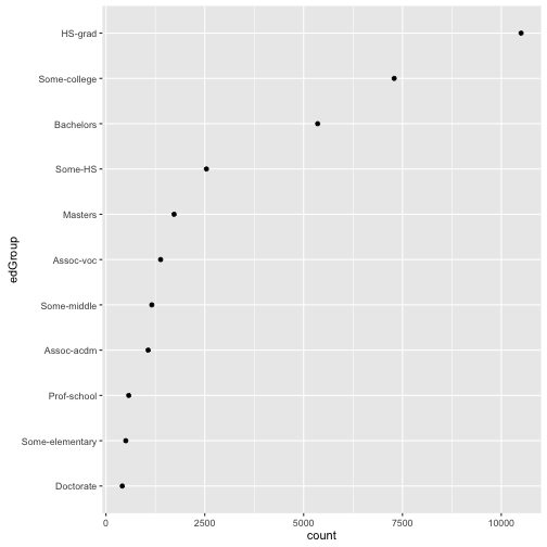 As you can see, pretty similar in idea and in execution. We can check the speed of each method.
library(profr)
datadr_prof <- profr(datadr_test())
dplyr_prof <- profr(dplyr_test())datadr took 0.9 seconds, while ddply took 0.22 seconds. That’s a 75.56% speedup over datadr in this example.
Takeaways
It seems like both datadr and dplyr have their benefits. Of course, this example is almost a joke because of everything is small enough to fit in memory. I’d like to test these packages on a much bigger dataset and see what I think after that. The ability of using Hadoop with datadr is an attractive one, although I don’t anticipate ever having me hands on data big enough to use it to it’s fullest capability. Both are interesting packages building on a sound principle and I look forward to using both more.
blog comments powered by Disqus