Watching: Neural networks
As part of the course Stat 503 I am taking this semester, I will be posting a series of responses to assigned course readings and videos. Mostly these will be my rambling thoughts as I skim papers.
This week we are watching some videos on neural networks from Andrew Ng, as well as Trevor Hastie and Robert Tibshirani (video 1 video 2 video 3 video4 video 5 video 6). These videos give a good introduction to the concepts behind neural networks, including the model representaion, motivation behind, and a detailed explanation of logistic regression.
A neural what what?
The term “neural network” for me evokes images of an incredibly complex model that is fit with some unknown blackbox procedure, probably in the cloud. Something like this.
In reality, a neural network is a highly flexible non-linear model that can be used for classification. The model uses multiple layers that are related to each other through sigmoid functions. Hence, a neural network is something like a nested logistic regression.
library(diagram)## Loading required package: shapelibrary(dplyr)
M <- matrix(nrow = 8, ncol = 8, data = 0) %>% data.frame()
names <- expand.grid(c("x", "{a^{(2)}} "), 1:3)
names <- bquote(.(parse(text = c(apply(names, 1, function(x) paste0(x[[1]], "[", x[[2]], "]")), "output", "h[Theta](x)"))))
M[,1] <- M[,3] <- M[,5] <- c(0, "", 0, "", 0, "", 0, 0)
M[,2] <- M[,4] <- M[,6] <- c(0, 0, 0, 0, 0, 0, "", 0)
M[,7] <- c(0, 0, 0, 0, 0, 0, 0, "")
pos <- matrix(c(c(0.10, 0.850),
c(0.4, 0.850),
c(0.10, 0.475),
c(0.4, 0.475),
c(0.10, 0.100),
c(0.4, 0.100),
c(0.65, 0.475),
c(0.9, 0.475)), ncol = 2, byrow = TRUE)
plotmat(M, pos = pos, name = names, lwd = 1, box.lwd = 2,
curve = 0, cex.txt = 0.8, box.size = 0.1,
box.prop = 0.5, arr.type = "triangle", arr.pos = .75)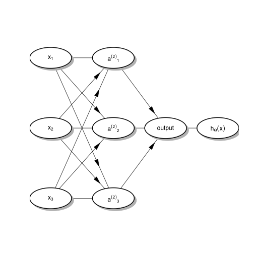
The model is thought of as being in three layers (from left to right): the visible layer, the hidden layer, and the output layer. The hidden layer activation nodes values \(a_i^{(2)}, i =1,\dots,3\) are each calculated as the sigmoid function of the linear combination of \(x_j\)’s. For example, \(a_i^{(2)} = g\left(\sum_{j=1}^3\theta^{(1)}_{ij}x_j\right)\) where \(g(x) = \frac{1}{1+e^{-x}}\). Then, at the output layer, each of these activation units is put together the same way to get \(h_\theta(x) = g\left(\sum_{j=1}^3\theta^{(2)}_{ij}a^{(2)}_j\right)\). In this way, neural networks are similar to inception.
Links to biology
Neural networks are so named because supposedly, this is what our brains do. They have neurons that have inputs and outputs and they connect to each other to relay messages. This ties to statistical learning in that it is thought that the neurons themselves can learn as well. So rather than having a set of neurons for everything we could want to do in life, we have a bunch of neurons that can learn everything we need to know, when we need it. Neural networks are so called because the algorithm was an attempt to mimic the brain.
As functional MRI and advanced brain imaging have improved, so has our understanding of the brain. However, when this methodology first became popular in the 1980s, however we knew a lot less about the brain (see here). As such, I think it’s fair to question whether a neural network actually does mimic the human brain, or whether it is just a catchy name for a very flexible non-linear classification model. I have to be honest, “neural network” does sound a whole lot more exciting!
blog comments powered by Disqus